Etienne Côme

Séminaire Labex Bezout, 14 Mai 2019
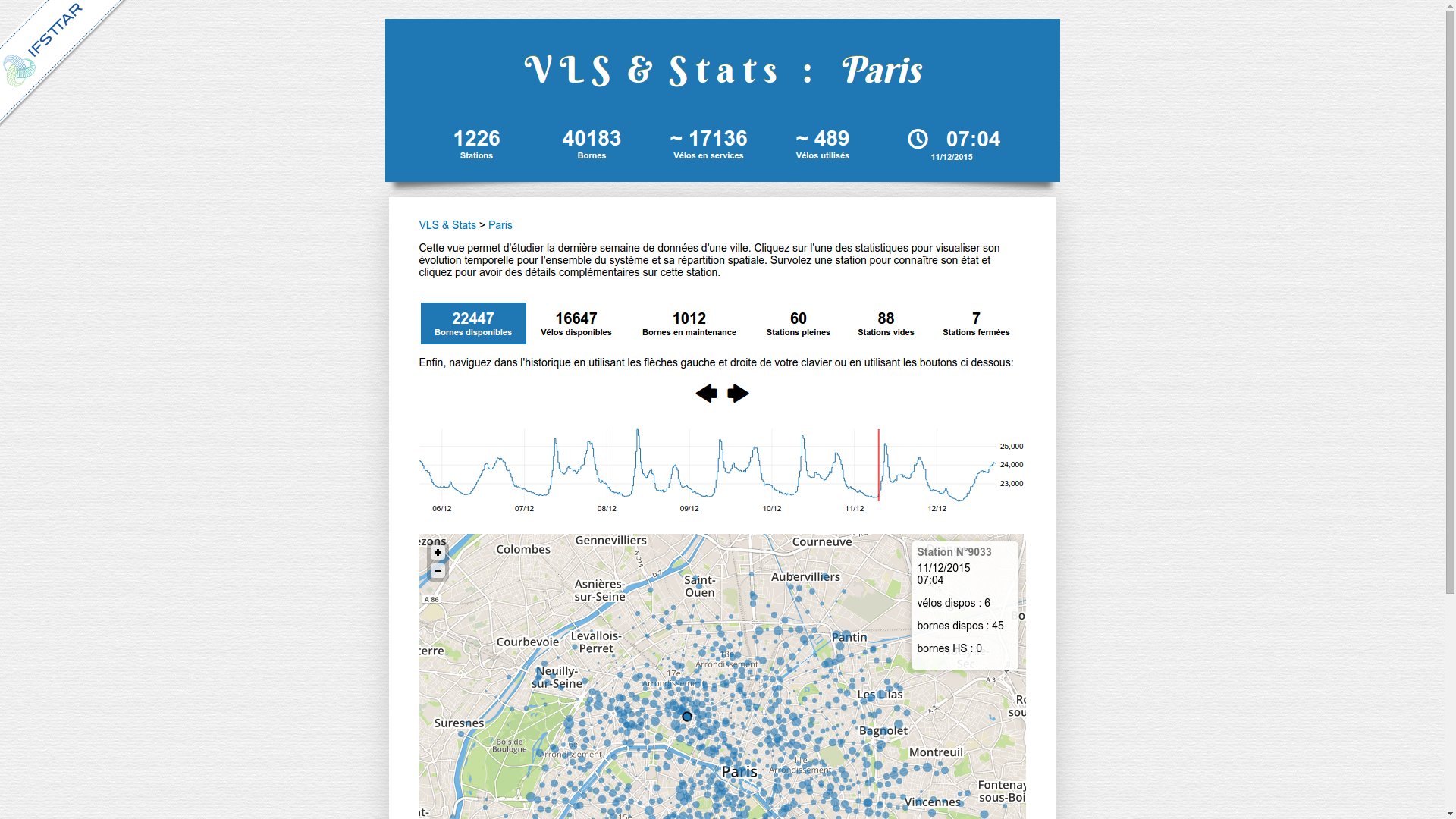
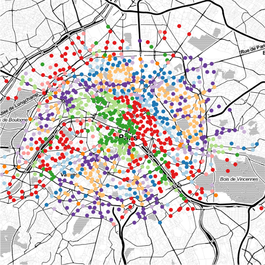
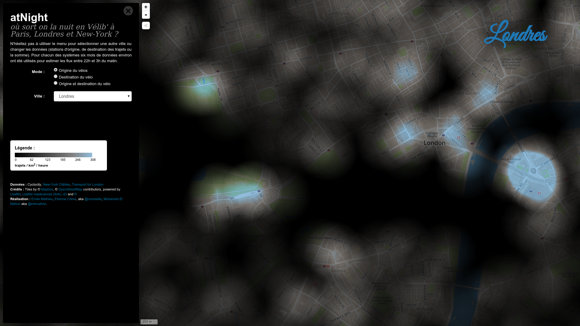
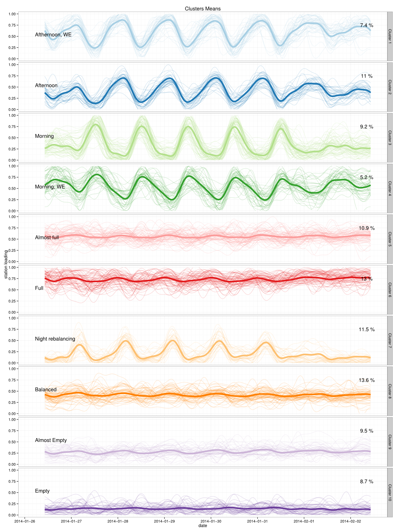 The Discriminative Functional Mixture Model for the Analysis of Bike Sharing Systems [preprint]
 The Discriminative Functional Mixture Model for the Analysis of Bike Sharing Systems [preprint]
 The Discriminative Functional Mixture Model for the Analysis of Bike Sharing Systems [preprint]

|

|

|

|

|

|

|

|
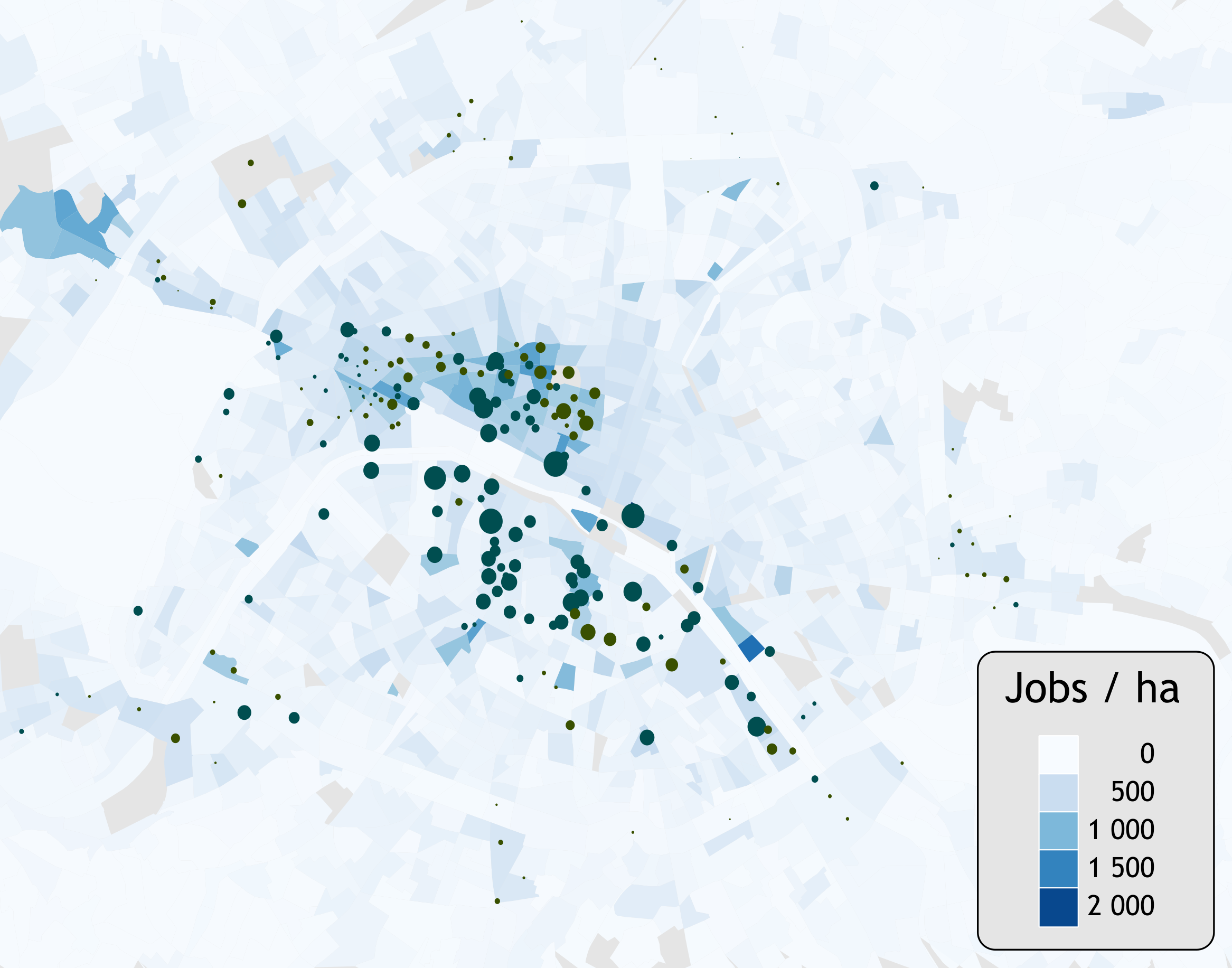
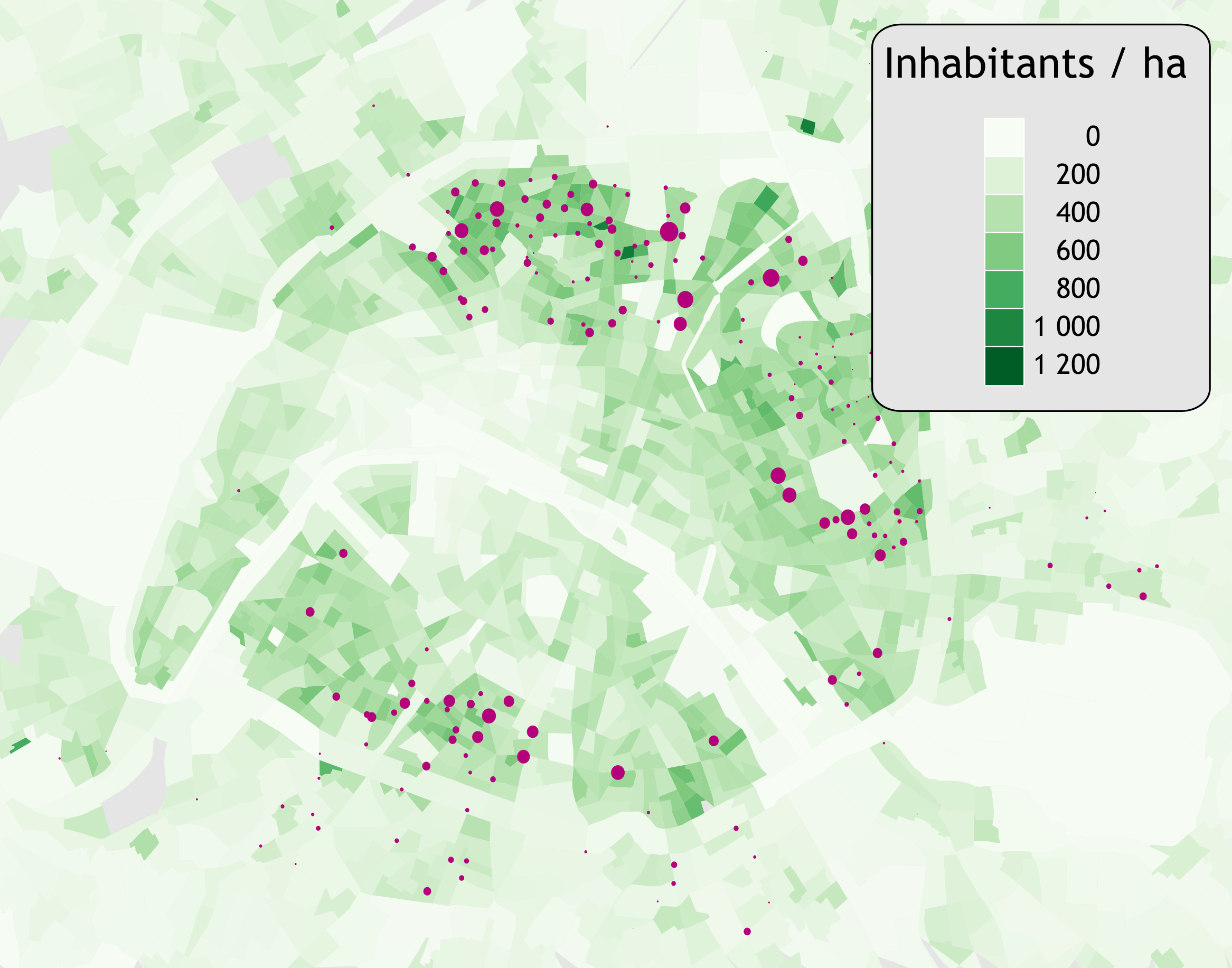
| hab/ha | emp/ha | serv/ha | com/ha | |
|---|---|---|---|---|
| * | 162 | 237 | 4.2 | 3.7 |
| Leisure (1) | 367 | 189 | 6.3 | 4.4 |
| Leisure (2) | 261 | 322 | 7.7 | 6.9 |
| Parks | 172 | 90 | 2 | 1.7 |
| Stations | 209 | 206 | 2.4 | 1.8 |
| 375 | 108 | 3.8 | 2.7 | |
| Jobs(1) | 138 | 409 | 4.5 | 2.8 |
| Jobs(2) | 157 | 456 | 5.7 | 5.6 |
| Average | 301 | 163 | 3.8 | 2.8 |
 Local stationarity of BSS behaviour / OD
Small bags of successive trips $\approx$ stationarity of OD
Documents (bags of words) = bags of successive trips (5000)
With :
Local stationarity of BSS behaviour / OD
Small bags of successive trips $\approx$ stationarity of OD
Documents (bags of words) = bags of successive trips (5000)
With :
 Model selection with perplexity analysis(clear drop for K=5)


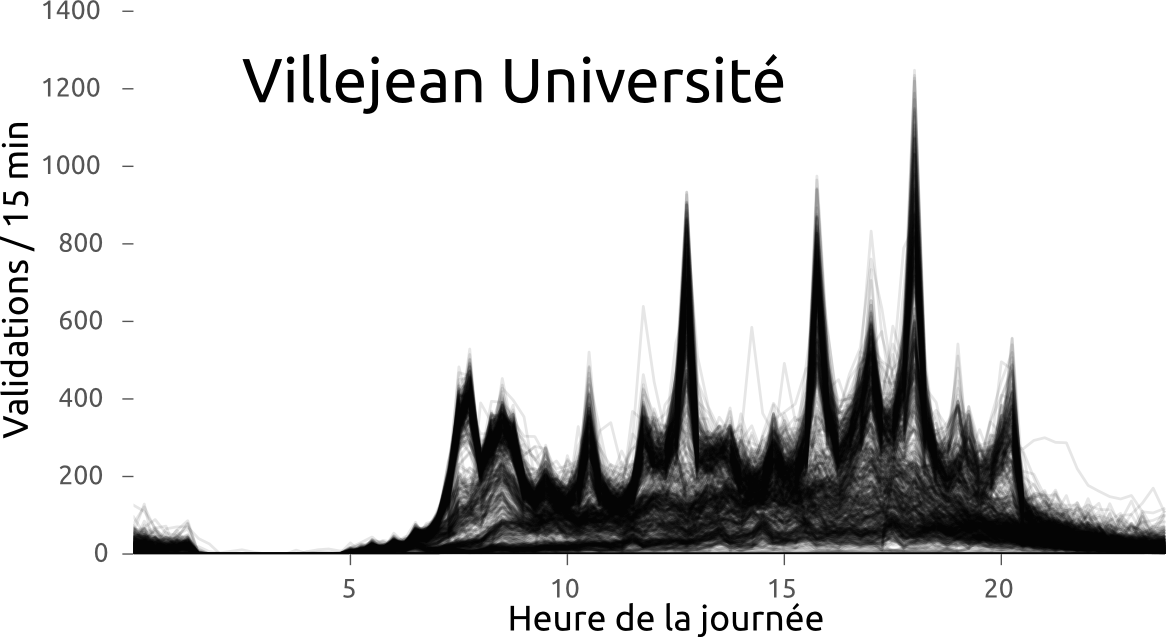
#Rennes #metro #Star des chaises jetées sur la ligne aérienne de métro à Villejean. Dégâts importants. Trafic interrompu pendant 2h?
— Samuel Nohra (@SamuelNohra) 29 mars 2016
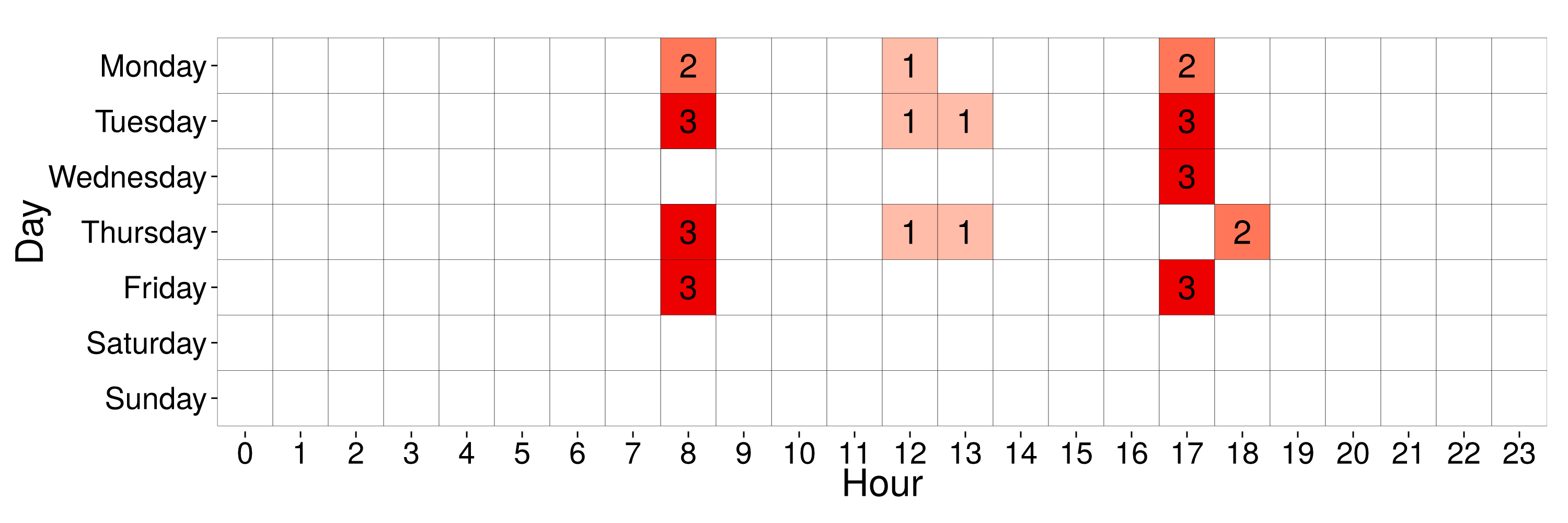
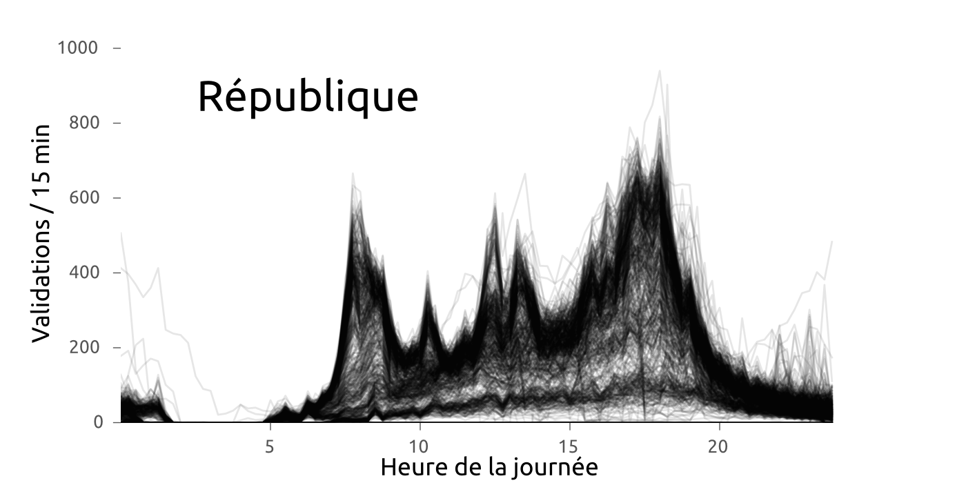
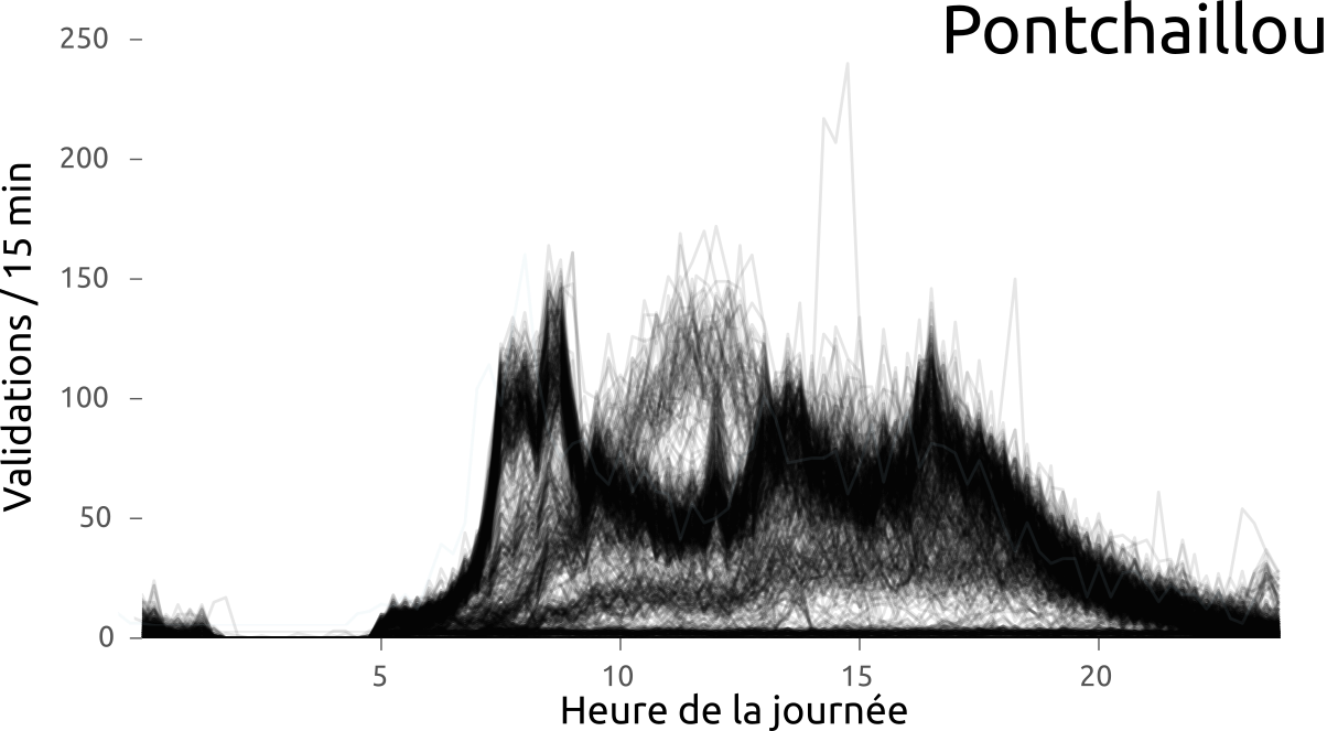
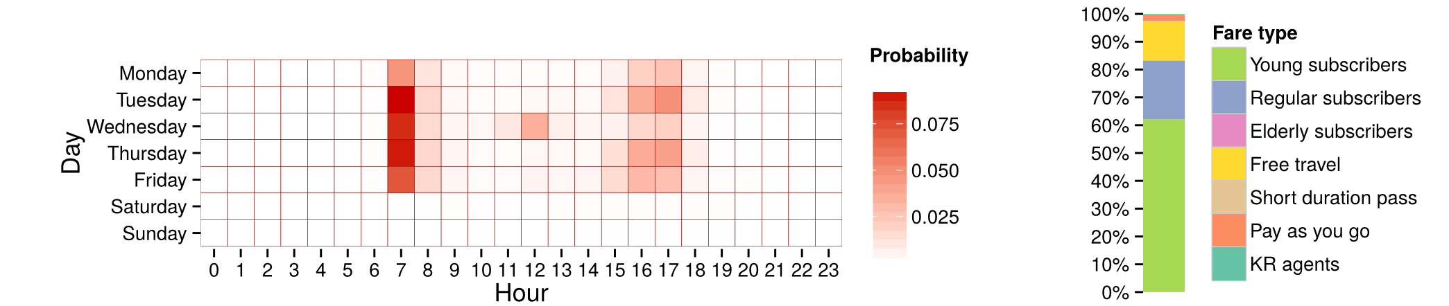
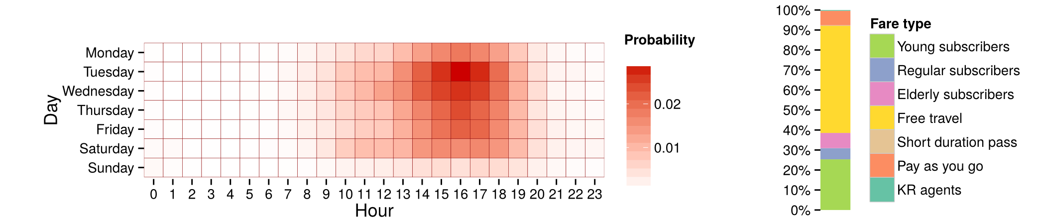
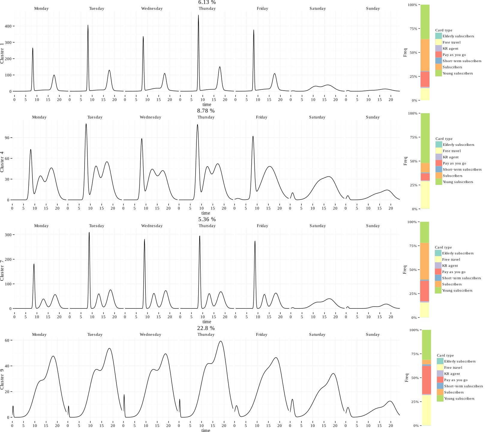
 Mean profile of a cluster with 4.55% of users
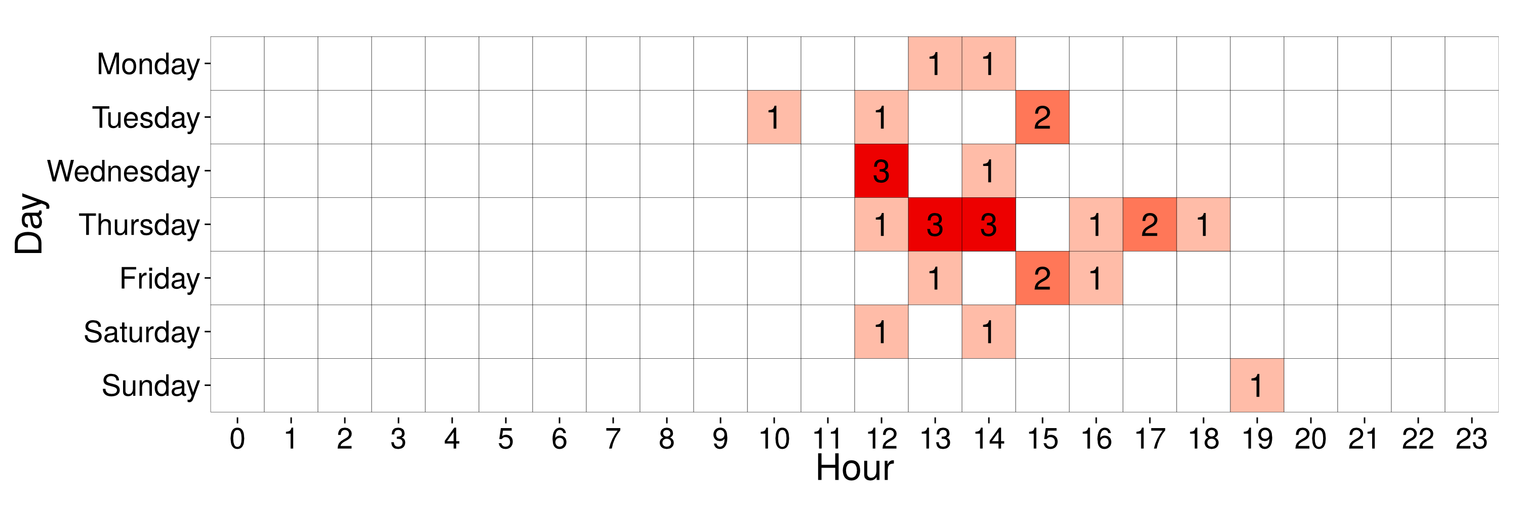
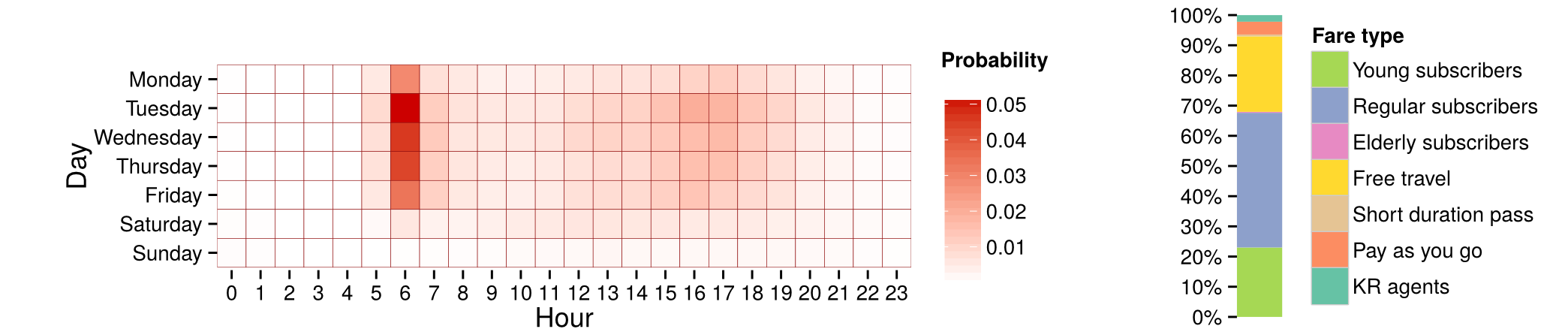
 Mean profile of a cluster with 12.54% of users
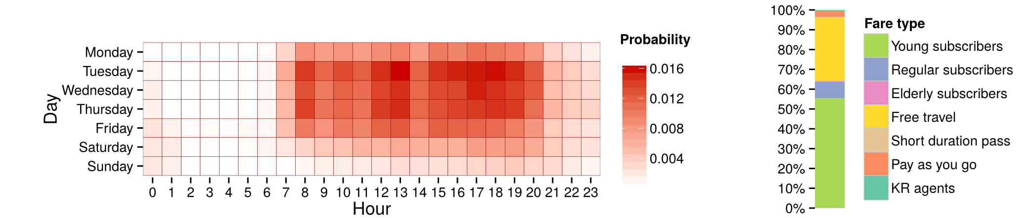
 Mean profile of a cluster with 3.6% of users
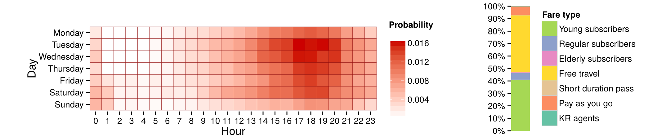
 Mean profile of a cluster with 15.13% of users
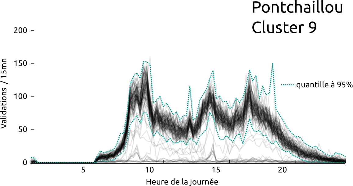
 Mean profile of a cluster with 6.44% of users
 Mean profile of a cluster with 8.64% of users
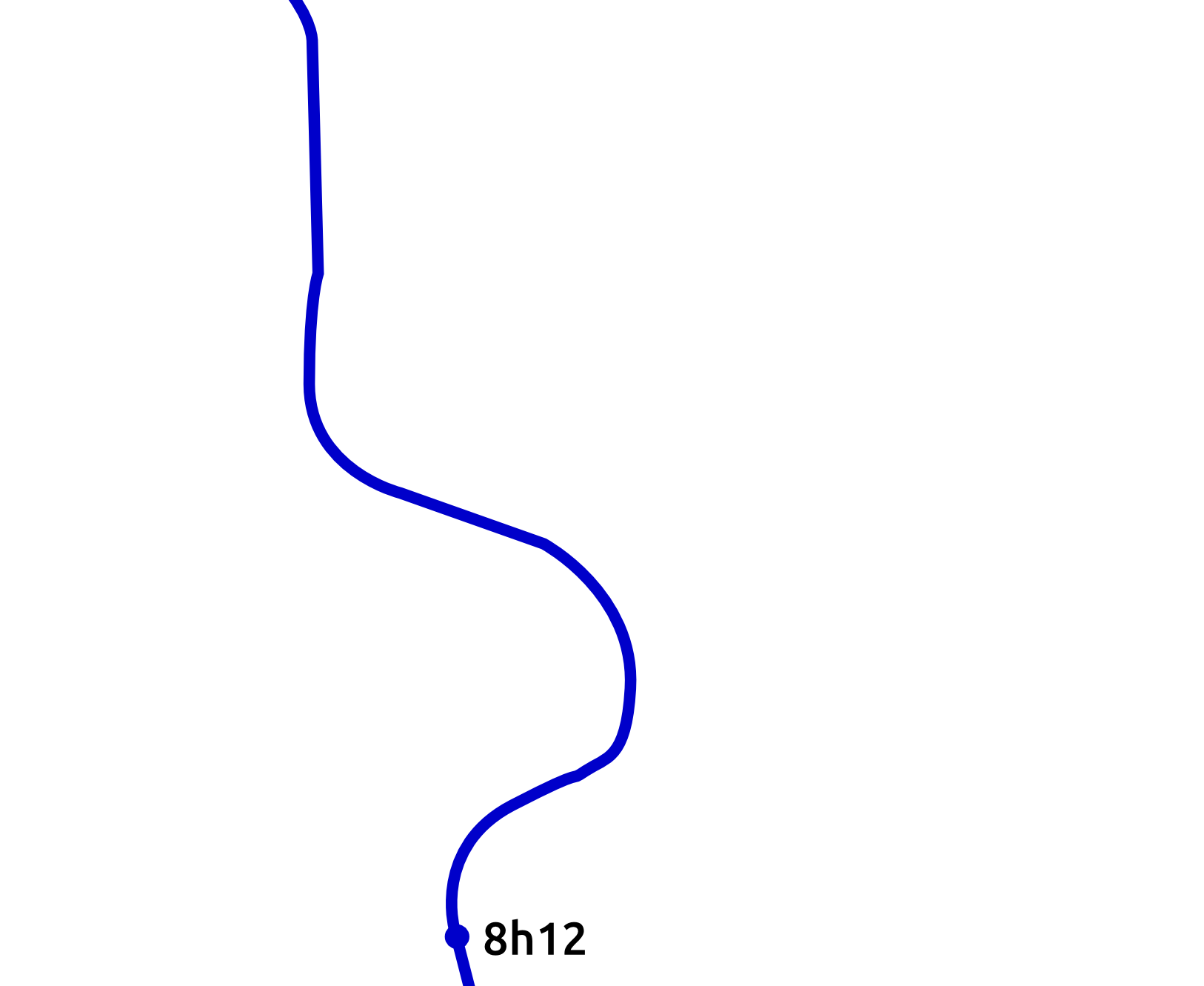
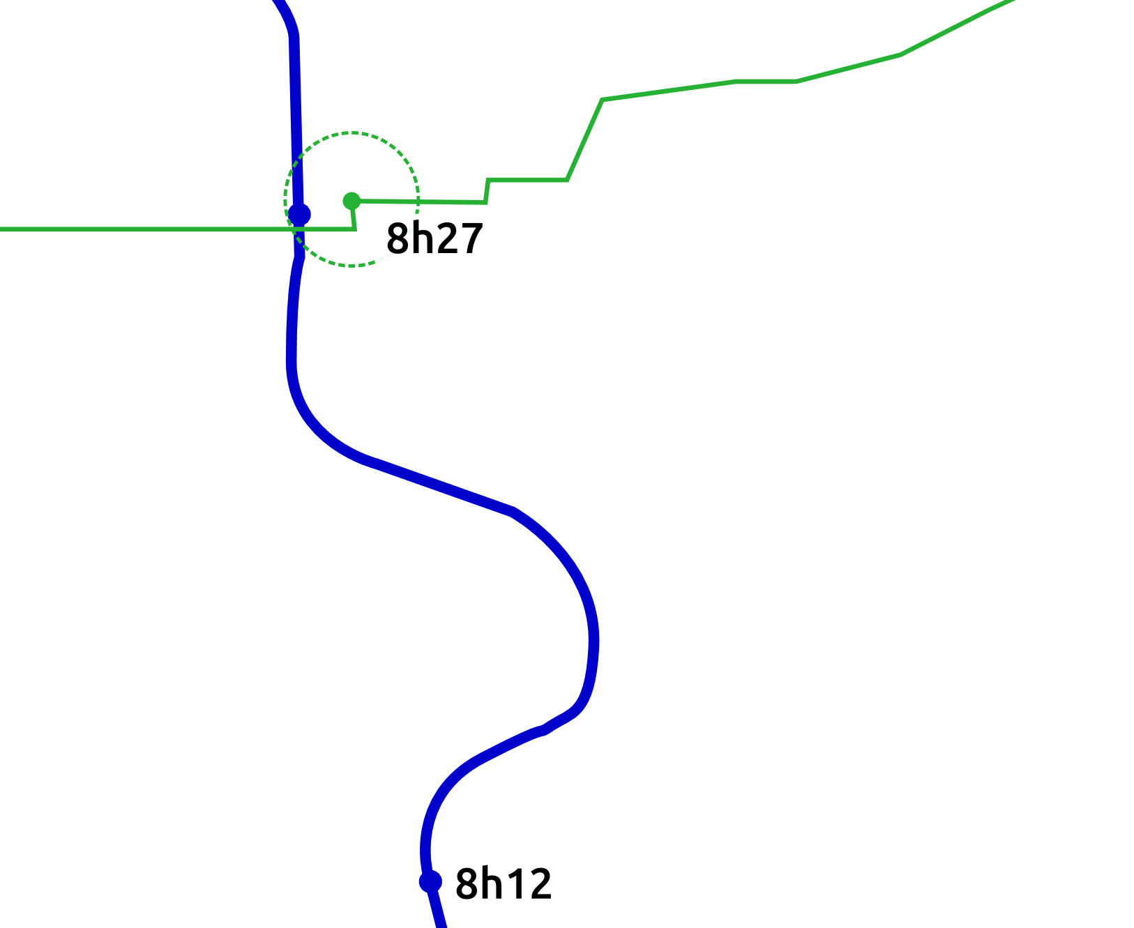
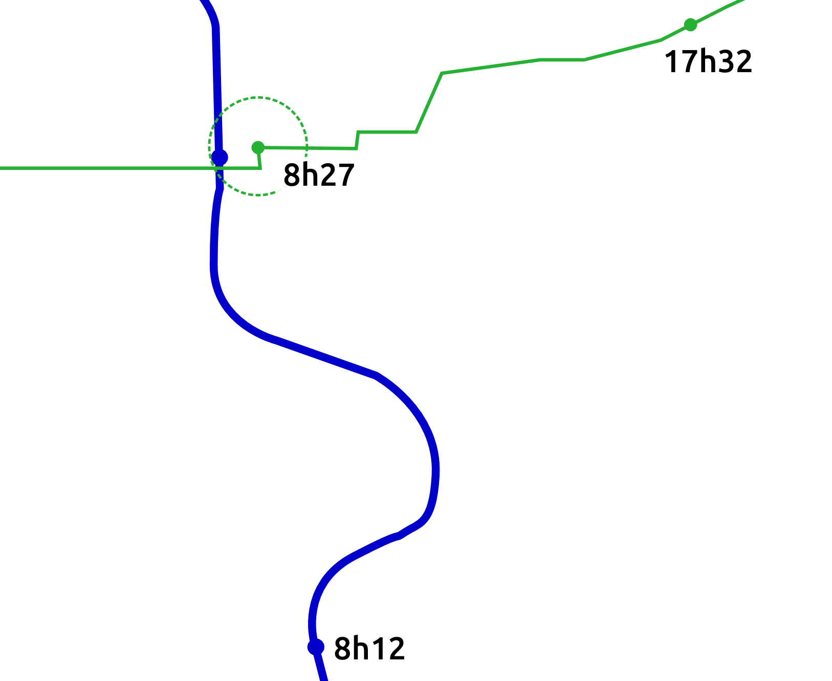
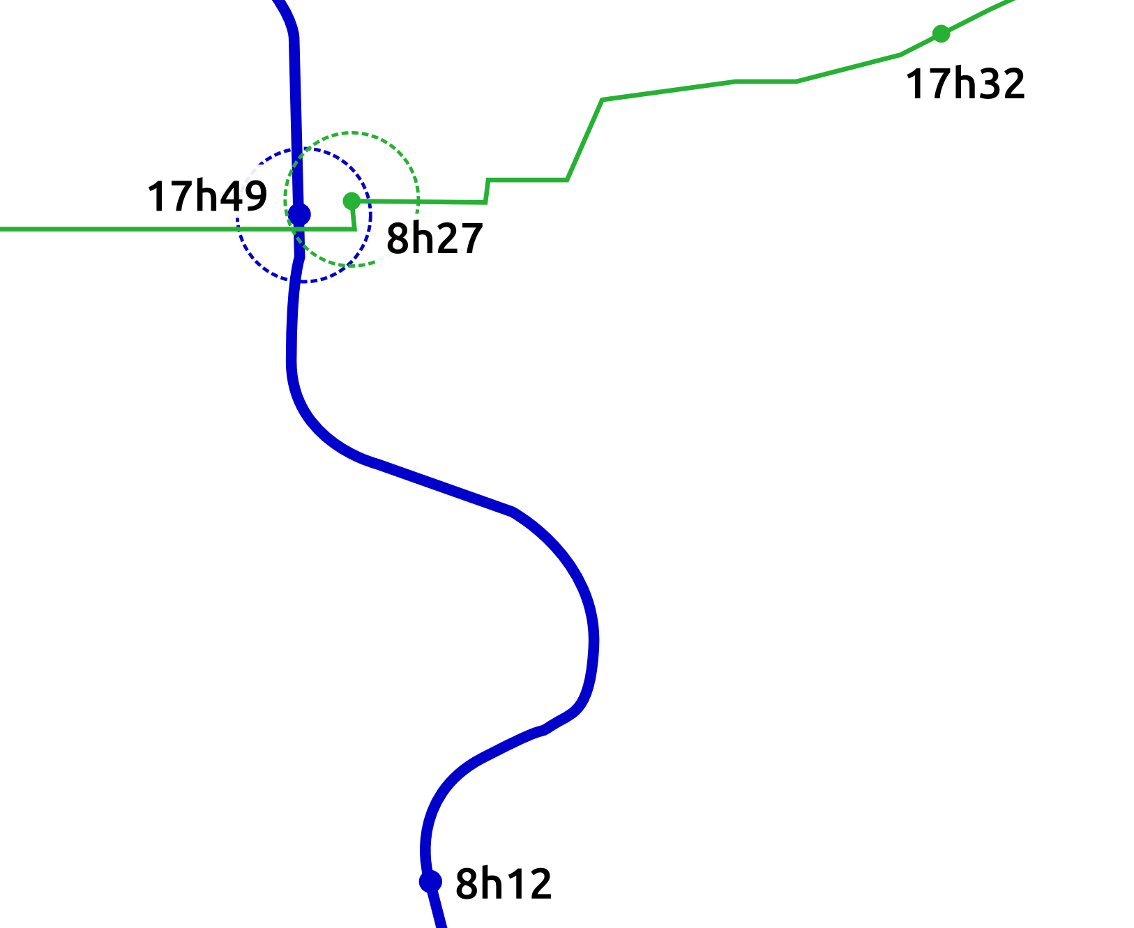
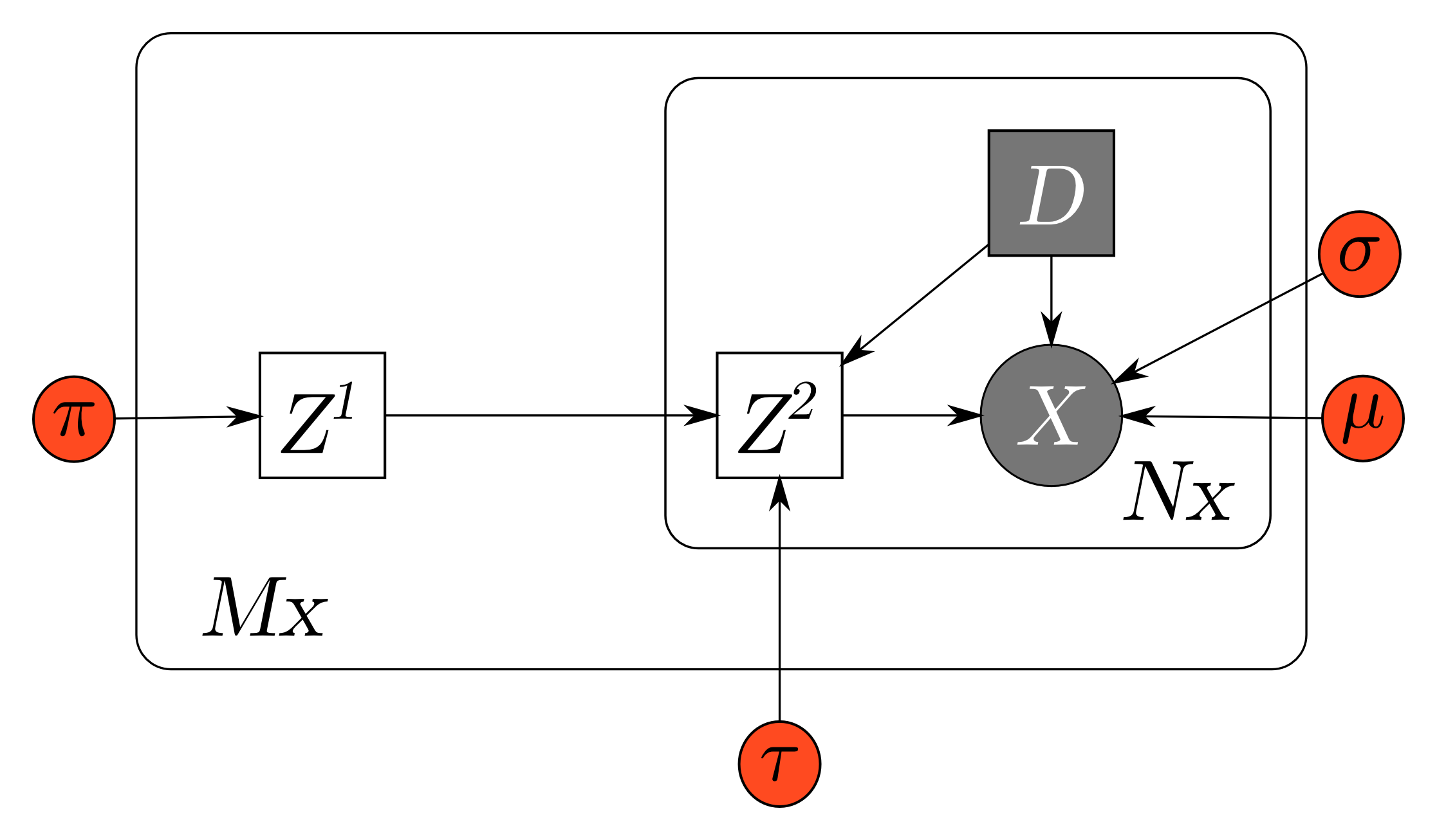 Generative model for continuous time user clustering
 simulated data
 simulated data
 simulated data
 simulated data
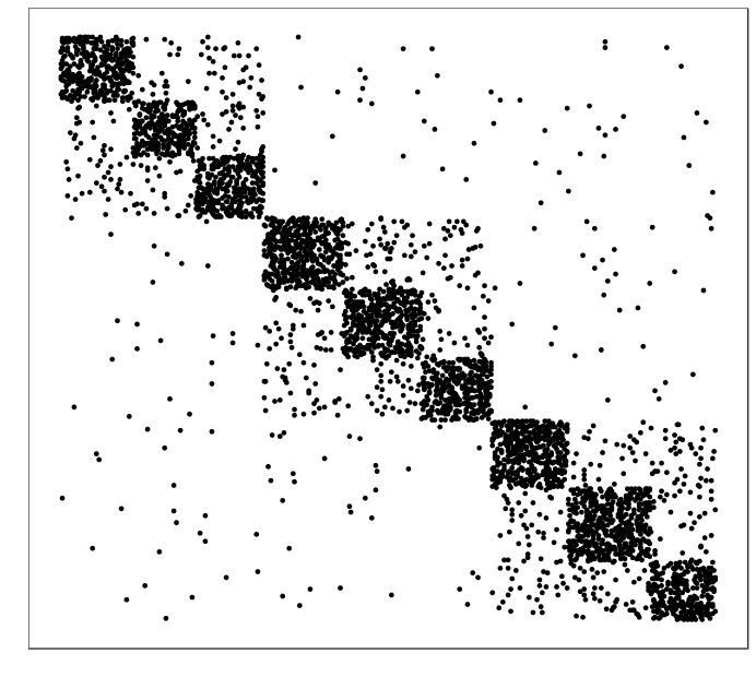
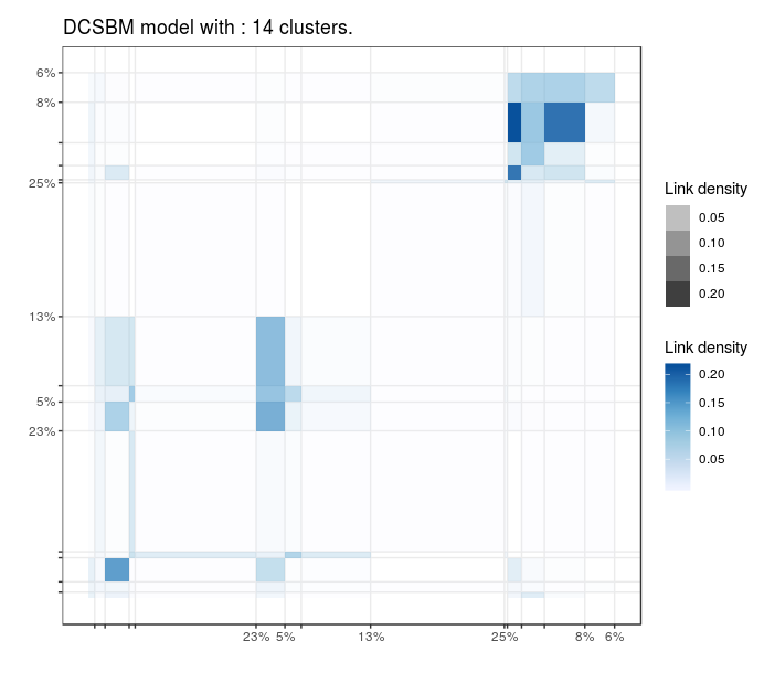
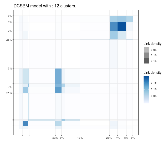
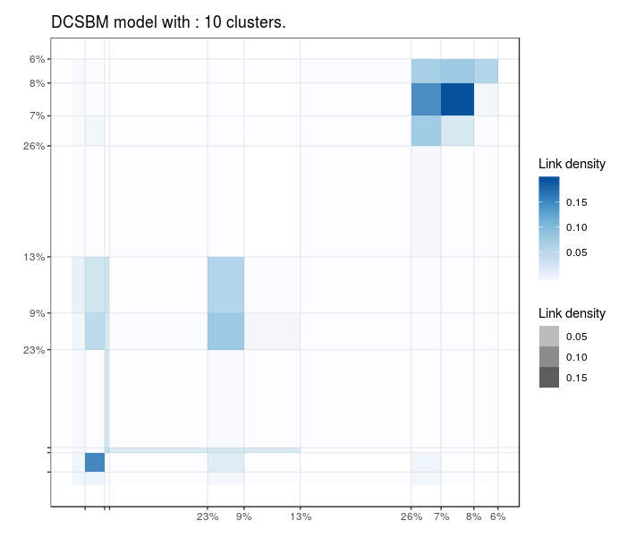
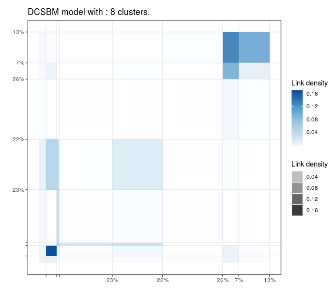
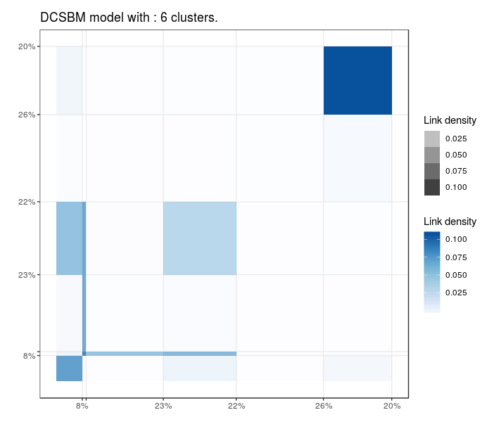
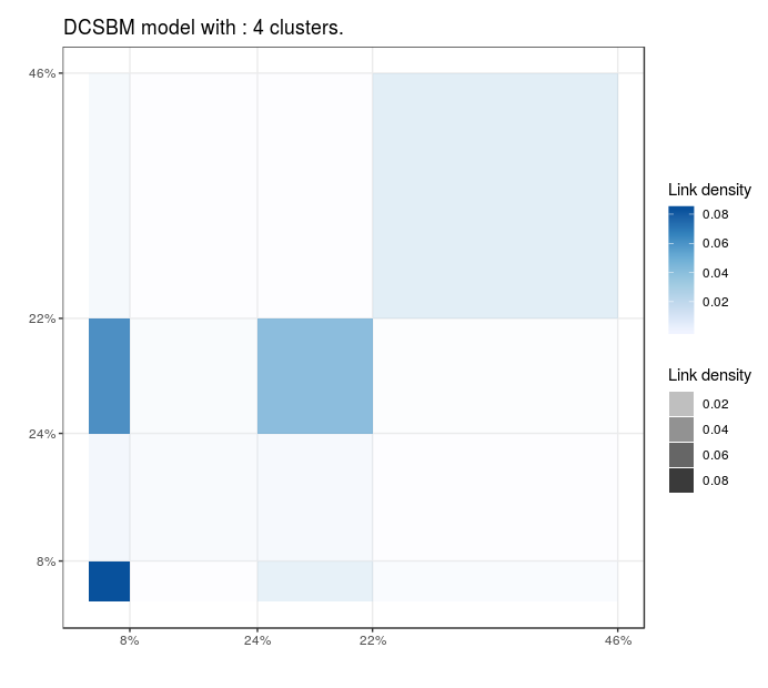
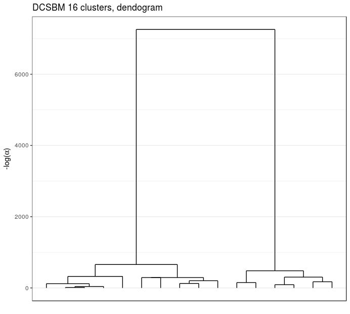 Blogs politiques (US)
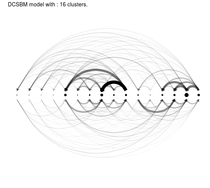 Blogs politiques (US)
 Blogs politiques (US)
 Blogs politiques (US)
 Blogs politiques (US)
 Blogs politiques (US)
 Blogs politiques (US)
 Blogs politiques (US)
 Blogs politiques (US)
 Blogs politiques (US)
 Blogs politiques (US)
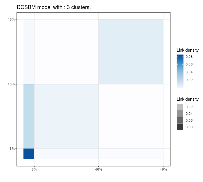 Blogs politiques (US)
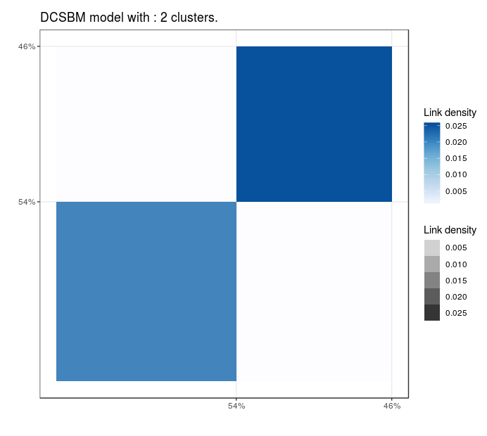 Blogs politiques (US)